Skyrmion collapse using NEB

using CairoMakie
using DelimitedFiles
using CubicSplines
using MicroMagnetic

In this example, we will compute the energy barrier of a skyrmion collapse into the ferromagnetic state using the NEB method. Firstly, we use create_sim method to describe the studied system. For example, the system is a thin film (120x120x2 nm^3) with periodic boundary conditions, and three energies are considered.

mesh = FDMesh(; nx=60, ny=60, nz=1, dx=2e-9, dy=2e-9, dz=2e-9, pbc="xy")
params = Dict(:Ms => 3.84e5, :A => 3.25e-12, :D => 5.83e-4, :H => (0, 0, 120 * mT))

Dict{Symbol, Any} with 4 entries:
  :A  => 3.25e-12
  :H  => (0, 0, 95493.0)
  :D  => 0.000583
  :Ms => 384000.0

Using NEB can be divided into two stages. The first stage is to prepare the initial state and the final state. We assume that the initial state is a magnetic skyrmion and the final state is ferromagnetic state.

In this method, we will obtain a magnetic skyrmion. The skyrmion state is saved as 'skx.vts'.

function relax_skx()
    function m0_fun_skx(i, j, k, dx, dy, dz)
        r2 = (i - 30)^2 + (j - 30)^2
        if r2 < 10^2
            return (0.01, 0, -1)
        end
        return (0, 0, 1)
    end

    sim = create_sim(mesh; m0=m0_fun_skx, params...)
    relax(sim; max_steps=2000, stopping_dmdt=0.01)
    save_vtk(sim, "skx")

    return sim
end

relax_skx (generic function with 1 method)

We will invoke the relax_skx method to obtain a magnetic skyrmion state and plot the magnetization.

sim = relax_skx()
plot_m(sim)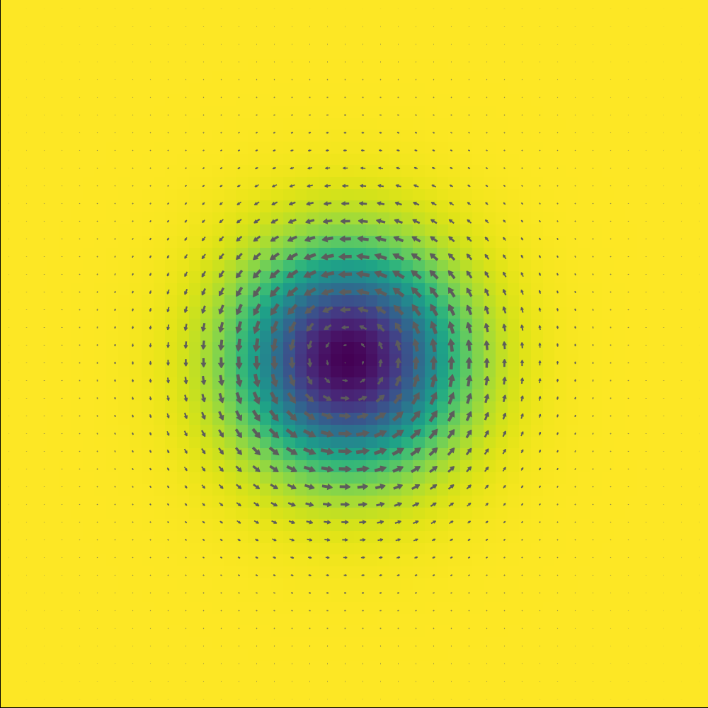

The following is the second stage.

We need to define the initial and final state, which is stored in the init_images list. Note that any acceptable object, such as a function, a tuple, or an array, can be used. Moreover, the init_images list could contain the intermediate state if you have one.

init_images = [read_vtk("skx.vts"), (0, 0, 1)];

We need an interpolation array to specify how many images will be used in the NEB simulation. Note the length of the interpolation array is the length of init_images minus one. For example, if init_images = [read_vtk("skx.vts"), read_vtk("skx2.vts"), (0, 0, 1)], the length of interpolation should be 2, i.e., something like interpolation = [5,5].

interpolation = [6];

To use the NEB, we use the create_sim method to create a Sim instance.

sim = create_sim(mesh; params...);

We create the NEB instance and set the spring_constant, the driver could be "SD" or "LLG"

neb = NEB(sim, init_images, interpolation; name="skx_fm", driver="SD");
````

neb.spring_constant = 1e7

Relax the whole system

julia relax(neb; stopping_dmdt=0.1, save_vtk_every=1000, max_steps=5000) ```

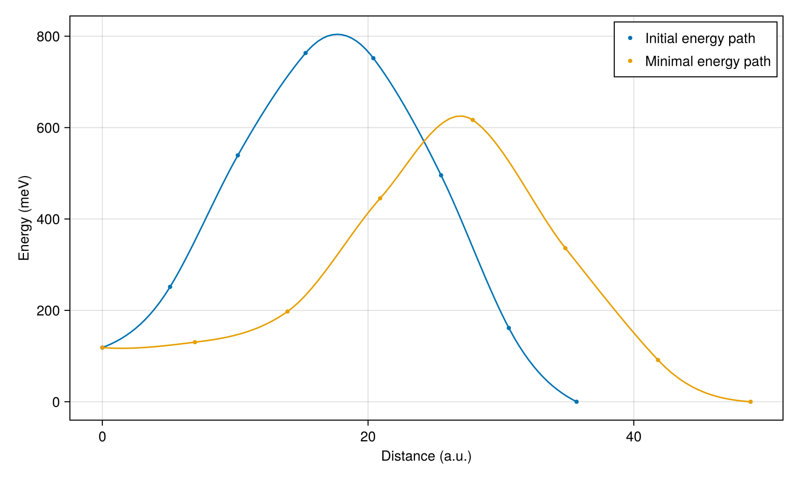
After running the simulation, the energy text file ('skx_fm_energy.txt') and the corresponding distance text file ('skx_fm_distance.txt') are generated.

We define a function to extract the data for plotting.

function extract_data(; id=1)
    energy = readdlm("assets/skx_fm_energy.txt"; skipstart=2)
    dms = readdlm("assets/skx_fm_distance.txt"; skipstart=2)
    xs = zeros(length(dms[1, 1:end]))
    for i in 2:length(xs)
        xs[i] = sum(dms[id, 2:i])
    end

    et = energy[id, 2:end]
    e0 = minimum(et)
    energy_eV = (et .- e0) / meV

    spline = CubicSpline(xs, energy_eV)

    xs2 = range(xs[1], xs[end], 100)
    energy2 = spline[xs2]

    return xs, energy_eV, xs2, energy2
end

function plot_energy()
    fig = Figure(; resolution=(800, 480))
    ax = Axis(fig[1, 1]; xlabel="Distance (a.u.)", ylabel="Energy (meV)")

    xs, energy, xs2, energy2 = extract_data(; id=1)
    scatter!(ax, xs, energy; markersize=6, label="Initial energy path")
    lines!(ax, xs2, energy2)

    xs, energy, xs2, energy2 = extract_data(; id=500)
    scatter!(ax, xs, energy; markersize=6, label="Minimal energy path")
    lines!(ax, xs2, energy2)
    #linescatter!(ax, data[:,2]*1e9, data[:,5], markersize = 6)
    #linescatter!(ax, data[:,2]*1e9, data[:,6], markersize = 6)

    axislegend()

    save("energy.png", fig)

    return fig
end

plot_energy()