Standard Problem 4

This example demonstrates how to simulate standard problem 4 using MicroMagnetic.jl. We start by relaxing the system to achieve a stable magnetization configuration, followed by applying an external magnetic field to study its effects.

Import necessary modules

using MicroMagnetic
using CairoMakie
using DelimitedFiles

Enable GPU acceleration

@using_gpu()

Define the system geometry: a film with thickness t = 3 nm, length L = 500 nm, and width d = 125 nm.

mesh = FDMesh(; nx=200, ny=50, nz=1, dx=2.5e-9, dy=2.5e-9, dz=3e-9);

Step 1: Relaxing the System

The first step in our simulation is to relax the system to obtain a stable magnetization configuration, often referred to as an "S" state. We encapsulate this process in the relax_system function.

function relax_system(mesh)
   sim = Sim(mesh; driver="SD", name="std4")

   Ms = 8e5
   A = 1.3e-11

   set_Ms(sim, Ms)   # Set saturation magnetization
   add_exch(sim, A)  # Add exchange interaction
   add_demag(sim)    # Add demagnetization

   init_m0(sim, (1, 0.25, 0.1))  # Initialize magnetization
   relax(sim; stopping_dmdt=0.01)  # Relax the system

   return sim
end

relax_system (generic function with 1 method)

The relax_system function takes a mesh as input and performs the following steps:

Simulation Initialization: The function initializes a simulation (sim) using the given mesh and sets the driver to "SD" (Steepest Descent), which is typically used for relaxation processes. The simulation is named "std4" for consistency with standard problem 4.

Material Parameters Setup: The saturation magnetization Ms and exchange constant A are set up using set_Ms and add_exch functions, respectively. Demagnetization effects are added using add_demag.

Initial Magnetization: The initial magnetization vector m0 is set using init_m0. In this case, it is initialized with a vector (1, 0.25, 0.1).

Relaxation: The system is relaxed using the relax function, which iteratively minimizes the system's energy until the change in magnetization (dm/dt) falls below a specified threshold (stopping_dmdt=0.01).

Relax the system to obtain a stable magnetization configuration

sim = relax_system(mesh);

[ Info: MicroSim has been created.
[ Info: Exchange has been added.
[ Info: Running Driver : MicroMagnetic.EnergyMinimization{Float64}.
[ Info: max_dmdt is less than stopping_dmdt=0.01 @steps=370, Done!

Step 2: Applying an External Field

After obtaining the stable "S" state, the next step is to apply an external magnetic field and observe the magnetization dynamics. Plot the magnetization distribution using the plot_m function

plot_m(sim; component='x')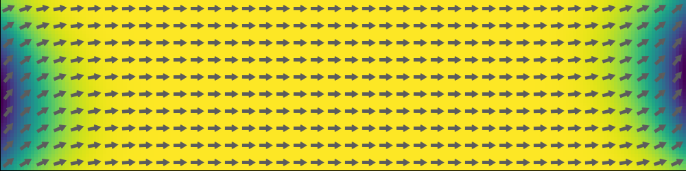

Apply an external field starting from the relaxed "S" state

set_driver(sim; driver="LLG", alpha=0.02, gamma=2.211e5)
add_zeeman(sim, (-24.6mT, 4.3mT, 0))  # Apply external magnetic field
if !isfile("std4.jld2")
   run_sim(sim; steps=100, dt=1e-11)  # Run the simulation for 10 steps
end

Step 3: Visualizing the Results

By default, run_sim generates a jld2 file, which stores the magnetization data. You can create a movie from this data to visualize the magnetization dynamics. Generate a movie based on the simulation results

jld2movie("std4.jld2"; output="assets/std4.mp4", component='x');
nothing #hide

TODO: check if gif can be used.