Nanobar

In this example, we consider a nanobar with dimensions 60nm x 10nm x 5 nm We used this example to demostrate how to obtain the magnetization distribution using MicroMagnetic.jl We first import MicroMagnetic and CairoMakie for plotting.

using MicroMagnetic
using CairoMakie

We create a FDMesh

mesh = FDMesh(; dx=2e-9, dy=2e-9, dz=2.5e-9, nx=30, ny=5, nz=2);

We create a Sim wth SD driver using Sim function and set the saturation magnetization Ms

sim = Sim(mesh; driver="SD")
set_Ms(sim, 8e5)   #Set saturation magnetization Ms=8e5 A/m

true

We consider two energies (i.e., exchange and demag) with exchange constant A = 1e-12 J/m.

add_exch(sim, 1e-12);   #Add exchange interaction
add_demag(sim);         #Add demagnetization

[ Info: Exchange has been added.

Initilize the magnetization to (1,1,0) direction,

init_m0(sim, (1, 1, 0))  #Initialize magnetization

true

We can plot the magnetization using plot_m function

plot_m(sim)

We relax the system to obtain the magnetization distribution. The stopping criteria is the stopping_dmdt, typically its value should be in the rangle of [0.01, 1].

relax(sim; max_steps=2000, stopping_dmdt=0.01)

[ Info: Running Driver : MicroMagnetic.EnergyMinimization{Float64}.
[ Info: max_dmdt is less than stopping_dmdt=0.01 @steps=88, Done!

We plot the magnetization again

fig = plot_m(sim)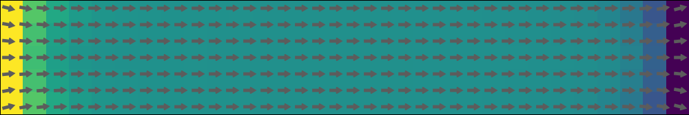

We save the figure to png.

save("bar.png", fig)

Save the magnetization state for later postprocessing, which can be visualization using Paraview (https://www.paraview.org/)

save_vtk(sim, "bar"; fields=["exch", "demag"])

Using the sim_with function.

We can use sim_with to simplify the setup of the simulation. We put all the parameters together:

args = (
    task = "Relax",
    mesh = FDMesh(dx=2e-9, dy=2e-9, dz=2.5e-9, nx=30, ny=5, nz=2),
    Ms = 8e5,
    A = 1e-12,
    demag = true,
    m0 = (1, 1, 0),
    stopping_dmdt = 0.01
);

then use the sim_with function

sim = sim_with(args);

[ Info: MicroSim has been created.
[ Info: Exchange has been added.
[ Info: Running Driver : MicroMagnetic.EnergyMinimization{Float64}.
[ Info: max_dmdt is less than stopping_dmdt=0.01 @steps=88, Done!

We plot the magnetization

plot_m(sim)