Standard Problem 4 (sim_with)
link: https://www.ctcms.nist.gov/~rdm/std4/spec4.html/
In this example, we demonstrate how to use MicroMagnetic.jl to simulate standard problem 4, which involves a thin film geometry. We will run the simulation on a GPU, process the results, and visualize the magnetization dynamics.
Import MicroMagnetic.jl
using MicroMagneticEnable GPU acceleration
@using_gpu()Define the system geometry: a film with thickness t = 3 nm, length L = 500 nm, and width d = 125 nm. Gather all the parameters related to standard problem 4:
args = (name="std4", task_s=["relax", "dynamics"],           # List of tasks
        mesh=FDMesh(; nx=200, ny=50, nz=1, dx=2.5e-9, dy=2.5e-9, dz=3e-9), Ms=8e5, # Saturation magnetization
        A=1.3e-11,                              # Exchange constant
        demag=true,                             # Enable demagnetization
        m0=(1, 0.25, 0.1),                      # Initial magnetization
        alpha=0.02,                             # Gilbert damping
        steps=100,                              # Number of steps for dynamics
        dt=0.01ns,                              # Time step size
        stopping_dmdt=0.01,                     # Stopping criterion for relaxation
        dynamic_m_every=1,                      # Save magnetization at each step
        H_s=[(0, 0, 0), (-24.6mT, 4.3mT, 0)]);
Run the simulation using the sim_with function:
sim = sim_with(args);[ Info: MicroSim (FD) has been created.
[ Info: Saturation magnetization has been set.
[ Info: Exchange has been added.
[ Info: Static Zeeman has been added.
[ Info: Running Driver : MicroMagnetic.SD{Float64}.
[ Info: max_dmdt is less than stopping_dmdt=0.01 @steps=370, Done!
[ Info: The driver LLG is used!
....................................................................................................
[ Info: step = 100 t = 1.000000e-09With the above code, the simulation for standard problem 4 is complete. Next, we proceed to process the data, such as visualizing the magnetization distribution or creating a movie from the simulation results.
We plot the time evolution of the magnetization using CairoMakie
using CairoMakie
fig = plot_ts("std4_llg.txt", ["m_x", "m_y", "m_z"];  xlabel="Time (ns)", ylabel="m", transparency=true)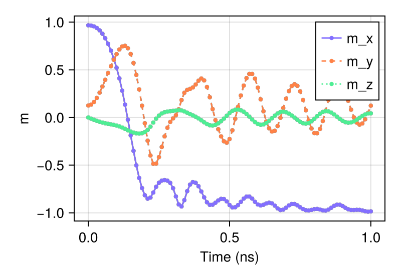
Generate a movie from the simulation ovfs stored in folder std4_LLG:
ovf2movie("std4_LLG"; output="../public/std4.mp4", component='x');