Stochastic LLG

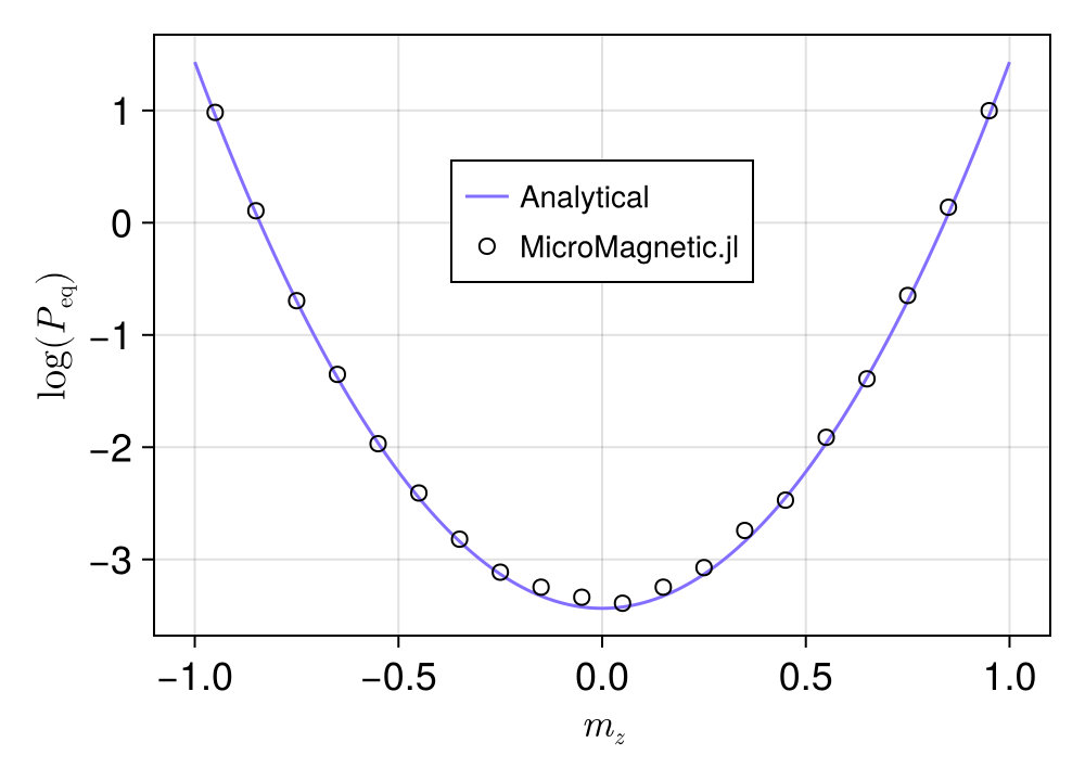
In this example, we will verify the thermal noise in SLLG, see Fig.6 script. We will then compare the distribution of magnetization with the analytical solution.

We import necessary packages.

using MicroMagnetic
using CairoMakie

@using_gpu()

We define a function to describe the simulation setup.

function run(; dt=1e-15)
    mesh = CubicMesh(; nx=30, ny=30, nz=30)

    V = 2.8e-26
    sim = Sim(mesh; driver="LLG", integrator="RungeKutta")
    sim.driver.alpha = 0.1
    sim.driver.gamma = 1.76e11
    sim.driver.integrator.step = dt

    #In principle, this value does not influence the result, however,
    #a large value will require a longer time to reach the equilibrium.
    set_mu_s(sim, 1.42e5 * V)

    init_m0_random(sim)

    add_anis(sim, 7.2e5 * V; axis=(0, 0, 1))
    add_thermal_noise(sim, 300.00)

    #dt = 1e-15, so the total time is 1e-15 * 1e5 = 1e-10 s
    relax(sim; max_steps=Int(1e5), stopping_dmdt=0, save_data_every=1000)

    save_vtk(sim, "sllg.vts")
    return sim
end

We define the analytical solution for the magnetization distribution.

using SpecialFunctions
function analytical()
    K = 7.2e5
    V = 2.8e-26
    T = 300
    chi = K * V / (k_B * T)
    Z = 2 * dawson(sqrt(chi)) / sqrt(chi)

    mzs = range(-1, 1, 201)
    ps = 1.0 / Z * exp.(-chi * (1 .- mzs .^ 2))
    return mzs, ps
end

To run the simulation and plot the distribution of magnetization, we define the following function. Note: the package StatsBase, SpecialFunctions and LinearAlgebra are required for this function.

using StatsBase
using LinearAlgebra
function run_and_plot()
    if !isfile("sllg.vts")
        run()
    end

    m = MicroMagnetic.read_vtk("sllg.vts")
    m = reshape(m, 3, div(length(m), 3))

    hist = fit(Histogram, m[3, :], -1:0.1:1; closed=:right)
    mz = midpoints(hist.edges[1])
    h = normalize(hist; mode=:pdf)

    fig = Figure(; size=(500, 360), fontsize=18)
    ax = Axis(fig[1, 1]; xlabel=L"$m_z$", ylabel=L"log($P_\mathrm{eq}$)")

    mzs, ps = analytical()
    l1 = lines!(ax, mzs, log.(ps); linestyle=:solid, color=:slateblue1, label="Analytical")
    s1 = scatter!(ax, mz, log.(h.weights); markersize=10, strokewidth=1, alpha=0,
                  color=:white, label="MicroMagnetic.jl")

    axislegend(ax; position=(0.5, 0.75), labelsize=14)

    save("P_mz.png", fig)
    return fig
end

Run the simulation and plot the distribution of magnetization

run_and_plot()

The plot should look like this: