Standard Problem 5
link: https://www.ctcms.nist.gov/~rdm/std5/spec5.xhtml
This script demonstrates the simulation of a rectangular film of magnetic material using MicroMagnetic.jl. The film has dimensions 100 nm × 100 nm × 10 nm. The simulation is divided into two main steps:
Relaxing the system to obtain an optimal energy state.
Simulating the dynamics of a vortex under an applied current.
using MicroMagnetic
using CairoMakie
using Printf
using DelimitedFiles

@using_gpu()
The system is a rectangular film of magnetic material with dimensions 100 nm × 100 nm × 10 nm.
mesh = FDMesh(; nx=20, ny=20, nz=2, dx=5e-9, dy=5e-9, dz=5e-9);Initialize a vortex roughly.
function init_fun(i, j, k, dx, dy, dz)
    x = i - 10
    y = j - 10
    r = (x^2 + y^2)^0.5
    if r < 2
        return (0, 0, 1)
    end
    return (-y / r, x / r, 0)
end
init_fun (generic function with 1 method)Step 1: Relax the system.
This function relaxes the system into an energy-optimal state using the steepest descent driver.
function relax_system(mesh)
    sim = Sim(mesh; driver="SD", name="std5")

    A = 1.3e-11  # Exchange constant
    Ms = 8e5     # Saturation magnetization
    set_Ms(sim, Ms)
    add_exch(sim, A)  # Exchange length=5.7nm
    add_demag(sim)

    init_m0(sim, init_fun)
    relax(sim; max_steps=10000, save_m_every=-1)

    return sim
end

sim = relax_system(mesh);
[ Info: MicroSim (FD) has been created.
[ Info: Saturation magnetization has been set.
[ Info: Exchange has been added.
[ Info: Running Driver : MicroMagnetic.SD{Float64}.
[ Info: max_dmdt is less than stopping_dmdt=0.01 @steps=174, Done!Plot the magnetization distribution using the plot_m function.
plot_m(sim; arrows=(30, 30), component='x')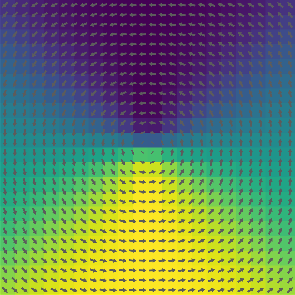
Step 2: Vortex Dynamics
We change the driver back to LLG and add spin transfer torques to the system.
set_driver(sim; driver="LLG", alpha=0.1, gamma=2.211e5)
add_stt(sim, model=:zhang_li, P=1.0, Ms=8e5, xi=0.05, J=(1e12, 0, 0))

# we add a SaverItem to save the guiding center each step
center = SaverItem(("cx", "cy"), ("<m>", "<m>"), compute_guiding_center)
run_sim(sim, steps=100, dt=5e-11, saver_item=center, save_m_every=1)
[ Info: The driver LLG is used!
[ Info: Zhang-Li Spin Transfer Torque has been added.
....................................................................................................
[ Info: step = 100 t = 5.000000e-09We plot the vortex center as a function of time.
fig = plot_ts("std5_llg.txt", ["cx", "cy"]; xlabel="Time (ns)", ylabel="Vortex center (nm)", y_units=[1e9, 1e9], transparency=true)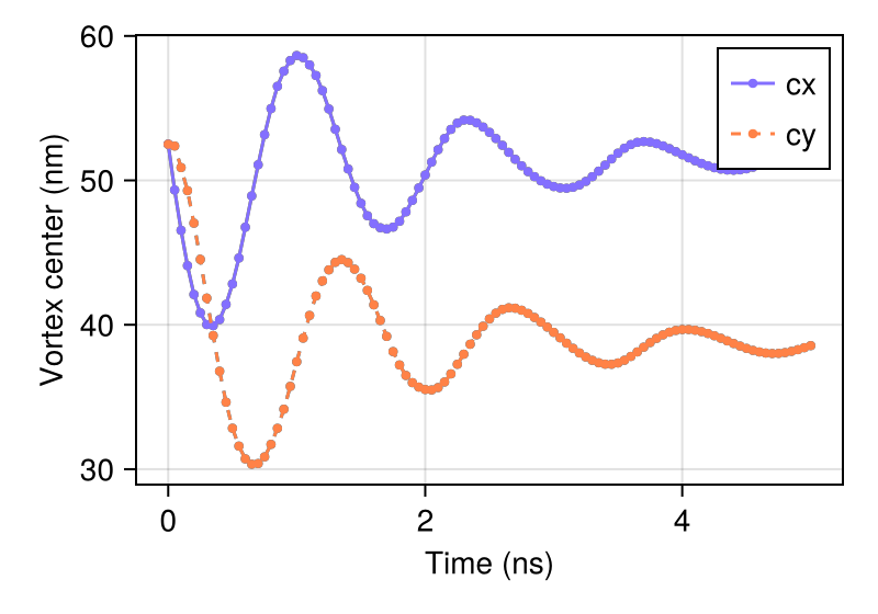
ovf2movie("std5_LLG"; output="../public/std5.mp4", component='x');