Demagnetizing Field Inside and Around a Uniformly Magnetized Sphere

In this example, we use the finite element method (FEM) to compute the demagnetizing field inside and around a uniformly magnetized sphere. It is well known that for a uniformly magnetized sphere with magnetization vector $\mathbf{M}=M_s{\mathbf{e}}_z$, the magnetic field inside the sphere is given by:

$${\mathbf{H}}_{\text{int}}=-\frac{1}{3}\mathbf{M}=-\frac{1}{3}{M}_s{\mathbf{e}}_z$$

Outside the sphere, the field is equivalent to that produced by a magnetic dipole with moment $\mathbf{m}=\mathbf{M}V$, where $V=\frac{4}{3}{R}_0^3$ is the volume of the sphere.

The corresponding magnetic scalar potential ${\varphi }_m$ satisfies:

$${\varphi }_m(\mathbf{r})=\{\begin{array}{ll}\frac{1}{3}\mathbf{M}\cdot \mathbf{R}& \text{inside the sphere}\\ \frac{1}{3}\frac{R_0^3}{R^3}\mathbf{M}\cdot \mathbf{R}& \text{outside the sphere}\end{array}$$

We begin by generating the simulation mesh using Netgen. The following sphere_air.geo file defines the geometry:

algebraic3d

solid sp = sphere(0, 0, 0; 10);

solid air = orthobrick(-2,-20,-20; 2, 20, 20) and not sphere(0, 0, 0; 12);

tlo sp -maxh=1.0;

tlo air -maxh=2.0;

This script creates:

• A solid sphere (sp) centered at the origin with radius 10

• An air box (air) that surrounds the sphere with a buffer region

• Different mesh sizes are assigned to the sphere (finer mesh) and air region (coarser mesh)

The resulting mesh looks like: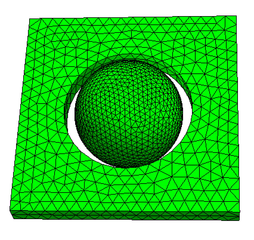

Note that the sphere and air are defined as separate solids. This allows the sphere to be labeled as region 1 and the air as region 2, enabling different material parameter assignments in subsequent simulations.

Simulation Setup

Import the necessary modules:

using MicroMagnetic
using Printf

Read the mesh file:

mesh = FEMesh("sphere_air.mesh")

A coarser sphere_air.mesh is available. Create a simulation object and set the saturation magnetization for region 1 (the sphere):

sim = Sim(mesh; driver="SD")
set_Ms(sim, 8e5, region_id=1)  # 800,000 A/m saturation magnetization

Set the initial magnetization direction and add the demagnetization energy term:

init_m0(sim, (0, 0, 1))  # Initial magnetization along z-axis

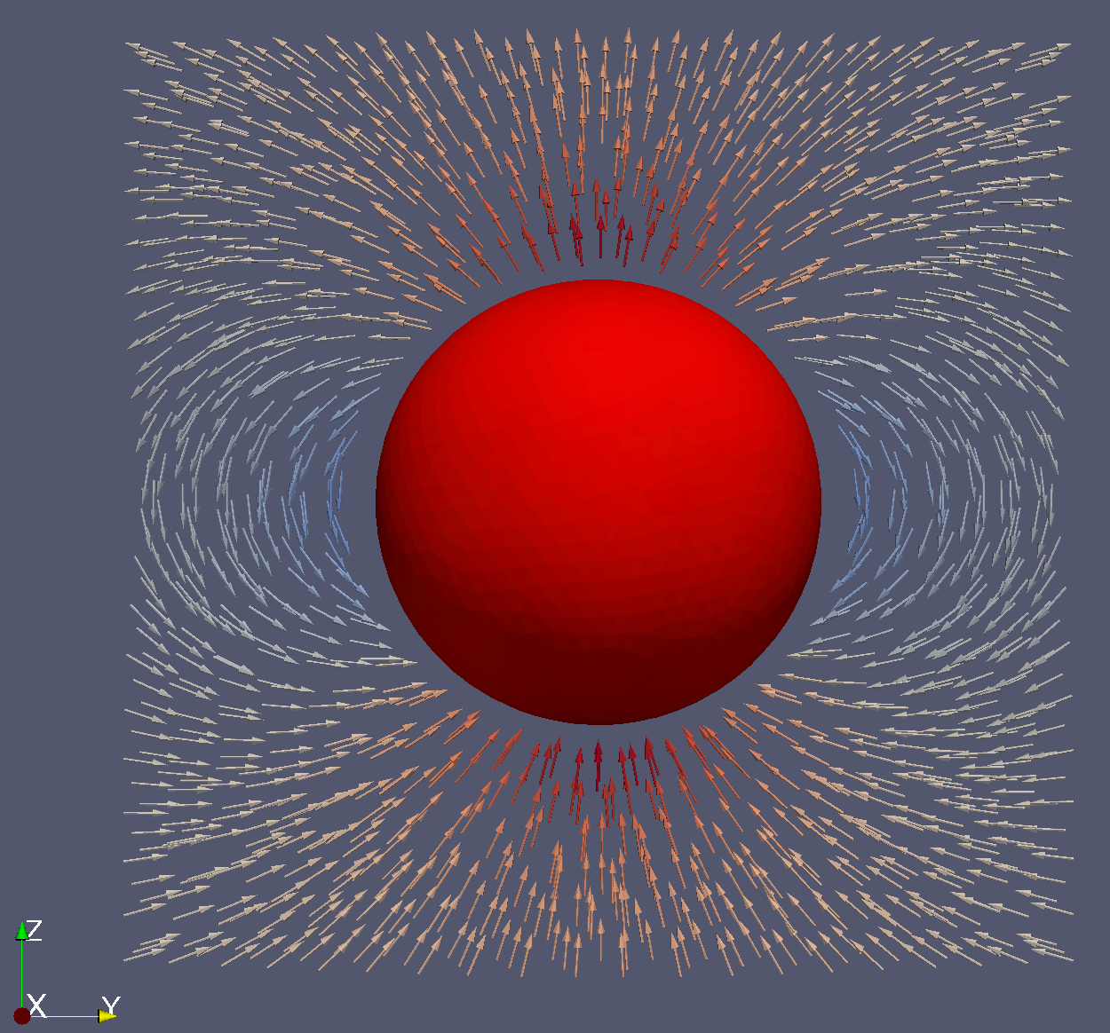
d = add_demag(sim, name="demag")  # Add demagnetization field calculation

Compute the effective field and save the results in VTK format for visualization:

MicroMagnetic.effective_field(sim, sim.spin)

save_vtk(sim, "sphere_demag.vtu", fields=["demag"])

The resulting VTU file can be opened in ParaView to visualize the magnetic field distribution around the sphere: